Hello, World in Qiskit

16-07-2021

Qiskit is a python SDK for simulating and running quantum algorithms on real quantum computers. As mentioned on qiskit.org:

Qiskit [kiss-kit] is an open-source SDK for working with quantum computers at the level of pulses, circuits and application modules.

I plan on writing a series of tutorials on getting started with quantum computing using qiskit, as I learn as well. Like any other programming tutorial, we start with a simple "Hello, world" program.

Measuring a quantum state

With conventional computers, the simplest program that one could perhaps make is printing out "hello, world". However, in contrast to this, in quantum systems, we go ahead and measure a quantum state (this seems to be the most rudimentary but complete program in quantum terms). Let's proceed to do just that!

Defining a quantum state

We import the necessary modules from Qiskit for this operation. To define a quantum circuit, we require the classes QuantumCircuit, QuantumRegister, ClassicalRegister and define a state variable psi as

\[ | \psi \rangle = \frac{1}{\sqrt{2}} \begin{pmatrix} 1\\ 1 \end{pmatrix} \]

Notice that the state \(| \psi \rangle\) is normalized. This is important, otherwise we'll end up with an error.

from qiskit import QuantumCircuit, QuantumRegister, ClassicalRegister
from math import sqrt

# define an initial state
psi = [1/sqrt(2), 1/sqrt(2)]

We then define a function prepare() which takes two parameters: a QuantumCircuit object named qc and the initial state psi. Remember that the quantum circuit that we define, only uses 1 qubit (notice the vector representation of \(| \psi \rangle\)).

def prepare(qc, psi):
    qc.initialize(psi, [0])     # [0] indicates the zeroth index (or) the first qubit

Python by default, calls by reference, so we don't have to worry about returning anything from prepare().

Building a quantum circuit

Let's proceed with making an actual quantum circuit. For this, we define a QuantumRegister object qr, which stores the qubits and a ClassicalRegister object cr which stores the measured values of those qubits.

qr = QuantumRegister(1)
cr = ClassicalRegister(1)

Combining the two registers, we now make a quantum circuit:

qc = QuantumCircuit(qr, cr)

Initializing and measuring the qubit

We then call our function prepare() to initialize the first qubit (the only qubit) of our quantum circuit qc.

prepare(qc, psi)

How do we go about measuring our state? That's where the ClassicalRegister object cr comes in. We use the measure method under the qc object to actually measure the qubit.

qc.measure(qr[0], cr[0])

The above syntax generally means that we're measuring the state of qr[0] (the first qubit) onto the classical register cr[0] where we store the measured value.

Visualizing the circuit

Ok so all of this is nice, but one can only describe so much. Let's see how our circuit actually looks like after applying the above operations. For this, we use the draw() method with the matplotlib backend.

>>> qc.draw(output='mpl')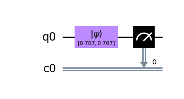

Choosing a backend for measurement

To measure the qubit and store the result in the classical register cr, we use the qasm_simulator backend. As we know from basic quantum mechanics,

from qiskit import Aer
backend = Aer.get_backend('qasm_simulator')

We then transpile our circuit for the qasm_simulator backend to understand and execute the circuit.

from qiskit import transpile
qc_compiled = transpile(qc, backend)

Now, we simply execute the circuit and gather the measurement results.

job = backend.run(qc_compiled, shots=1024)  # shots is the number of times we run the experiment
results = job.result()

We store the value of the result object and can further access the number of times we end up with a certain value of expected outcome with the get_counts() method.

counts = results.get_counts(qc_compiled)
print(counts)

{'0': 518, '1': 506}

Here we end up with a dictionary of key values '0' and '1', which indicate the following quantum states:

\[ | 0 \rangle = \begin{pmatrix} 1\\ 0 \end{pmatrix} \qquad | 1 \rangle = \begin{pmatrix} 0\\ 1 \end{pmatrix} \]

As expected, we get a 50-50 distribution of the states \(|0\rangle\) and \(|1\rangle\), since our starting state was \(|\psi\rangle\). We can also calculate this probability via the inner-product,

\[ |\langle 0 | \psi \rangle|^2 = \frac{1}{2} \qquad |\langle 1 | \psi \rangle|^2 = \frac{1}{2} \]

Let's visualize this in the form of a histogram. For this, we import the plot_histogram function.

>>> from qiskit.visualization import plot_histogram
>>> plot_histogram(counts)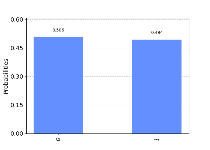

You can find the entire script in this gist.